경희대학교 허선영 교수님의 운영체제 수업을 기반으로 정리한 글입니다.
Preemptive & Nonpreemptive Scheduling
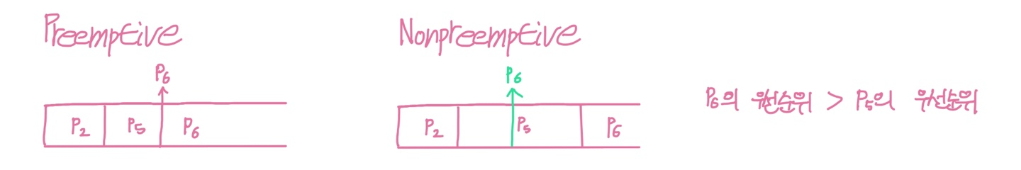
1. Nonpreemptive
: 기존 프로세스 내쫓지 않고, 종료 or 대기까지 기다림
2. Preemptive
: 기존 프로세스 내쫓음
-> race condition
Scheduling Criteria
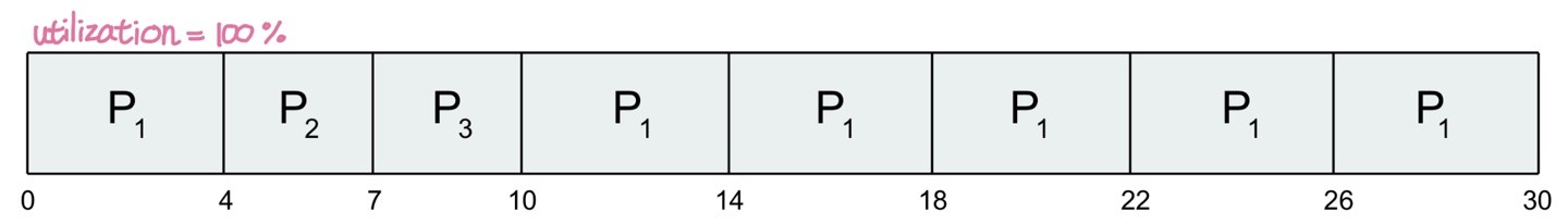
+ CPU Utilization
: CPU가 busy 유지하도록 100% 이용
+ Throughput: 단위시간 동안 완료한 프로세스 개수
-> 클수록 좋음
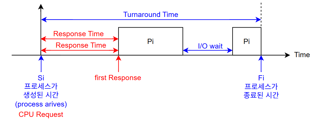
- Turnaround Time: process 생성부터 종료까지의 시간
- Waiting Time: ready queue
- scheduling affects only
- Response Time: CPU에 처음 할당되기까지의 시간 (the first response is produced)
-> 작을수록 좋음
Scheduling Algorithms
1. First-Come First-Served (FCFS) Scheduling
: CPU를 request 한 순서대로 스케줄링 with FIFO queue (nonpreemptive)
- convoy effect (호위 효과)
- short process behind long process
- Burst Time(CPU 이용 시간)이 긴 process가 먼저 도착할 경우, average waiting time 증가
-> CPU-bound, I/O-bound process 고려 필요
- CPU-bound: CPU Burst가 높은 long process
- I/O-bound: CPU Burst가 낮은 short process
2. Shortest-Job-First (SJF) Scheduling
: CPU Burst가 짧은 순서대로 스케줄링 (nonpreemptive)
- CPU Burst 예측 어려워 사용하지 않음
+ CPU Burst 예측 가능하다는 가정 하에, Optimal in terms of average waiting time
Determining Next CPU Burst Length
: exponential averaging (이전 burst length 이용하여 예측)
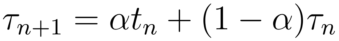
- T: 예측 값
- t: 실제 측정 값
※ preemptive version: shortest-remaining-time-first scheduling
3. Shortest Remaining Time First (SRTF) Scheduling
: Preemptive version of SJF scheduling (preemptive)
Example)
| Process | Arrival Time | Burst Time |
| P1 | 0 | 8 |
| P2 | 1 | 4 |
| P3 | 2 | 9 |
| P4 | 3 | 5 |

- Average wainting time = [(17 - 0 - 8) + (5 - 1 - 4) + (26 - 2 - 9) + (10 - 3 - 5)] / 4 = 6.5
time 계산
- wainting time = turnaround time - burst time
- turnaround time = finishing time - arrival time
P arrives or terminates -> Scheduling
4. Round-Robin (RR) Scheduling
: FCFS + time slice(quantum, 양자) (preemptive)
+ wait time에 bound 생겨 시간 보장 가능

+ request(CPU core 할당) 처음으로 response 하는 시간 줄어듦 (SJF보다 좋음)
- higher average turnaround than SJF
- q is too small -> context switch time 증가
- q is too large -> FCFS로 회귀
Example)
Time quantum = 4
| Process | Burst Time |
| P1 | 24 |
| P2 | 3 |
| P3 | 3 |
- 같은 process이면 context switching X
- but, timer interrupt는 계속 발생 (new process 확인 위해)
turnaround time varies with the time quantum
5. Priority Scheduling
: Priority number (integer) 순서대로 스케줄링 (우선순위 동일할 경우엔 FCFS)
- Problem: Starvation
- Solution: Aging (우선순위 증가)
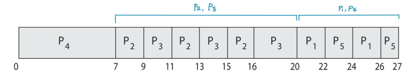
Example)
Time quantum = 2
| Process | Burst Time | Priority |
| P1 | 4 | 3 |
| P2 | 5 | 2 |
| P3 | 8 | 2 |
| P4 | 7 | 1 |
| P5 | 3 | 3 |
6. Multi-level Queue Scheduling
: 우선순위별로 ready queue 여러 개 사용
multilevel queue schedular defined by:
- number of queues
- scheduling algorithms for each queue
- scheduling among the queues
7. Multi-level Feedback Queue Scheduling
: multilevel queue + 큐 간 이동 가능
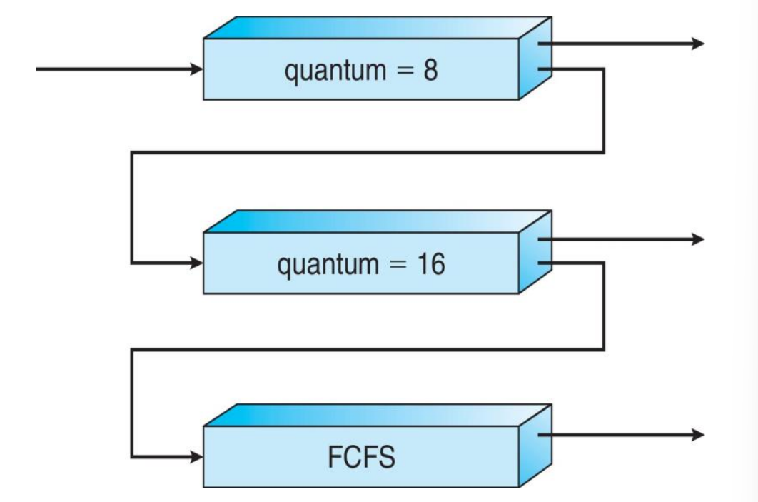
큐 간 이동
- aging: 우선순위 높아짐
- time quantum 동안 finish X -> 우선순위 낮아짐
Multi-Processor Scheduling
Multiprocessing architectures
1. Multiple CPUs
2. Multithreaded cores
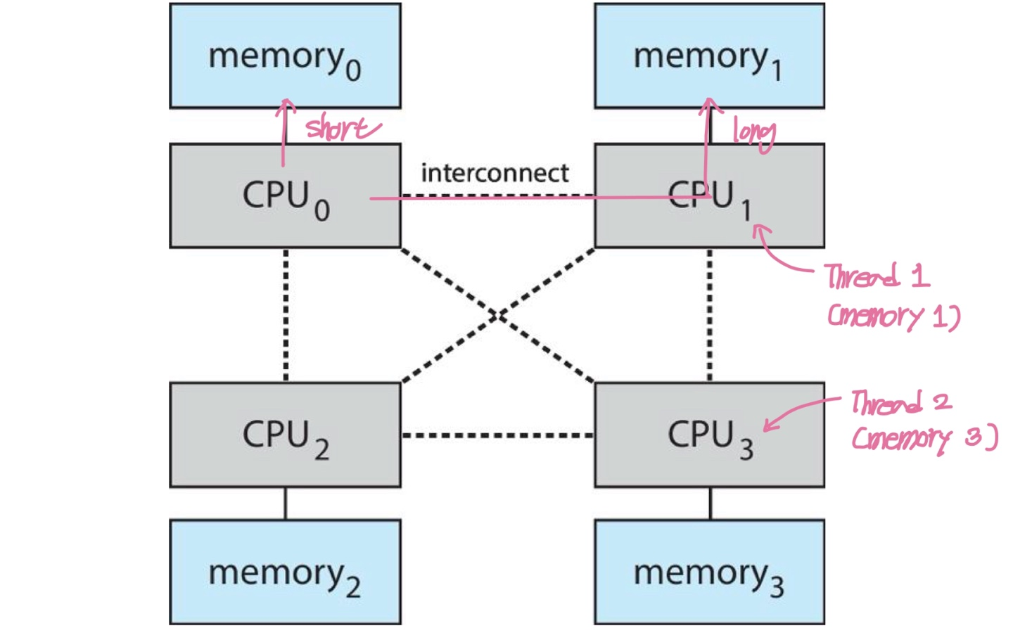
3. NUMA (Non-Uniform Memory Access) systems
: CPU마다 메모리가 근접하게 따로 달려있음
-> 데이터 위치에 따라 가져오는 시간이 다르기에 스레드를 많이 사용하는 메모리에 근접한 CPU에 두는 게 합리적인 스케줄링
4. Heterogeneous multiprocessing (종류가 다른)
: 코어 성능 다름
ex) Mobile System - ARM.Big.Litttle: 멀티 코어인데 하나는 Big(전력, 성능 높음), 하나는 Little(전력, 성능 낮음, 절전모드)
Multiple-Processor
Symmetric Multiprocessing (SMP)
: 코어별로 필요한 task 가져가 스케줄링

Multicore Processors
: 코어마다 하나의 thread 실행 가능
-> multi-processor 보다 multi-core가 전력, 속도 면에서 더 좋음

memory stall: 메모리 기다리는 시간
- 사칙연산, 레지스터 접근: 1 cycle
- 메모리 접근: 100 cycle (memory stall)
Multithreaded Multicore System
: If one thread has a memory stall, switch to another thread (hyperthreading)

hyperthreading: 하나의 core에서 이루어짐
Chip-multithreading (CMT)
: hyperthreading

▶ physical core / logical core
- physical cores: 실제 코어 개수
- logical cores: 실제 코어 개수 + 코어 처리할 수 있는 스레드 개수
Two levels of scheduling
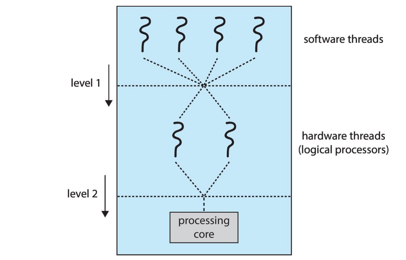
※ software threads: program, e.g., pthread 등 thread API
Multi-Processor Scheduling
Load Balancing
: 각각의 CPU에 주어지는 task 양 균등하게 분배
load balancing approaches:
- Push migration: OS schedular가 각 프로세서의 load를 주기적으로 확인하고 overloaded CPU에서 다른 CPU로 task push
- Pull migration: 쉬고 있는(idle) 프로세서들이 busy 프로세서로부터 waiting task pull
Processor Affinity
: 한 thread가 하나의 프로세서를 점유해 실행되고 있을 때, 해당 코어의 cache는 실행 중인 thread의 데이터 저장
-> 이를 thread가 해당 프로세서에 affinity(친밀도)를 갖는다고 표현함
Problem: load balancing을 통해 thread들이 여러 프로세서를 이동하면서 실행될 때, 친밀도와 상관없는 프로세서를 할당받으면 다시 해당 프로세서의 cache에 thread가 사용하는 데이터를 저장해야 하는 overhead 발생
-> Solution: affinity를 갖는 프로세서에서 다시 실행되게 함
- Soft affinity: 노력
- Hard affinity: 보장
Real-Time CPU Scheduling
: Deadline 존재
-> preemptive, priority-based scheduling
ex) 항공 시스템, 자율주행차 (safety-critical)
- Soft real-time systems: deadline priority 높음
- Hard real-time systems: 반드시 deadline 안에 끝내야 함

※ real-time CPU scheduling을 지원하는 대표 OS: RTOS (Hard의 경우 추가 알고리즘 필요)
Periodic Task Scheduling

- 0 <= t <= d <= p
- t: processing time (burst time)
- d: (relative) deadline
- p: period
1. static priority: Rate Monotonic (RM)
2. dynamic priority: Earlist Deadline First (EDF) -> process 도착 시점에 따라 결정
Rate Monotonic Scheduling
: shorter periods = higher priority, longer periods = lower priority
Example 1)
| Process | Period (= Deadline) | Processing Time |
| P1 | 50 | 20 |
| P2 | 100 | 36 |

Example 2)
| Process | Period | Processing Time |
| P1 | 50 | 25 |
| P2 | 80 | 35 |
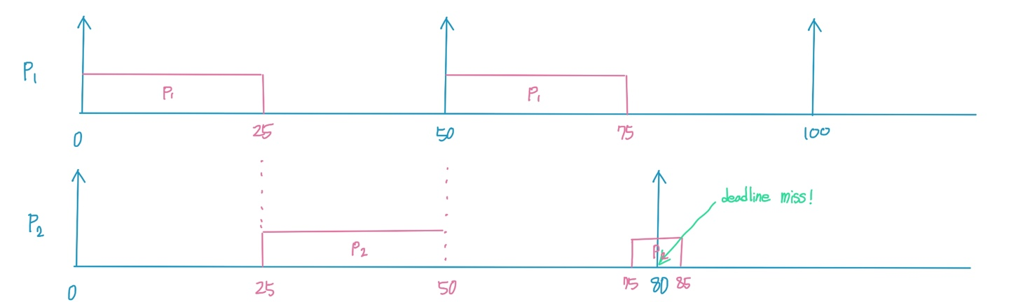
-> The rate monotonic is infeasible (사용 불가능한)
Earlist Deadline First Scheduling (EDF)
: earlier deadline = higher priority, later deadline = lower priority
Absolute Deadline vs Relative Deadline
- Absolute Deadline: 도착 시간 + relative deadline -> 동일한 process에 대해서도 인스턴스마다 Absolute Deadline 다름
- Relative Deadline: 도착 후 주어진 시간의 양
Example)
| Process | Period | Processing Time |
| P1 | 50 | 25 |
| P2 | 80 | 35 |

Algorithm Evaluation
Deterministic Modeling
: workload에 대해 criteria로 평가
- workload: period, deadline, processing time 등
- criteria: average waiting time 등
'CS > 운영체제' 카테고리의 다른 글
| Chapter 4: Thread & Concurrency (0) | 2025.05.06 |
|---|---|
| Chapter 3: Processes (0) | 2025.05.04 |
| Chapter 2: Operating System Structures (1) | 2025.05.04 |
| Chapter 1: Introduction (0) | 2025.05.04 |