경희대학교 박제만 교수님의 자료구조 수업을 기반으로 정리한 글입니다.
Heap
A heap is a binary tree that satisfies these special SHAPE and ORDER properties:
- Shape: Heaps' shape must be a complete binary tree. (위쪽, 왼쪽부터 채움)
- Order: Parents value > Child values (MAX heap)

▶ Heap Example
- Largest (Smallest) Value in a Heap -> root
BST와 Heap은 비슷한 듯 다르니, 구분할 수 있어야 한다.
- Heap: 부모 >= 자식
- BST: 왼쪽 서브트리 < 노드 < 오른쪽 서브트리
※ MAX heap <-> MIN heap

▶ Array Representation of Heaps
- complete binary tree -> array! (minimized empty space)
- 위에서 아래로, 왼쪽에서 오른쪽으로 번호를 붙임
array이기에 linked structure로 구현한 것에 비해 확장성이 떨어진다.
Heap Operations
Insert a New Node


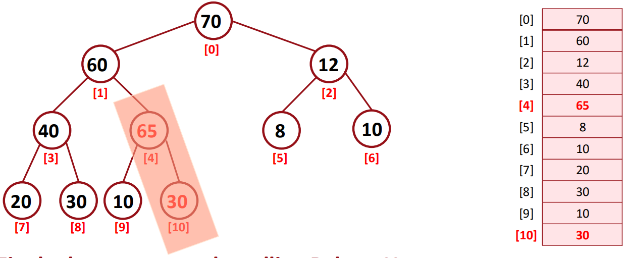


▶ Logical Level - insertItem(65)
- 1. Insert the new element in the next bottome leftmost place -> shape 만족
- 2. Fix the heap property by calling ReheapUp -> order 만
- If heap property is violated (chile> parent) -> Swap nodes

▶ reheapUp() - Implementation Level
- root: root의 idx
- boottom_id: 현재 비교하는 값의 idx
Why Do We Need a Heap?
- find max (or min) in root -> O(1)
- e.g., priority queue
※ 메모리 공간 heap 과는 아무런 상관이 없다. (just 이름만 같음)
※ priority_dequeue()
template<class ItemType>
bool QueueType<ItemType>::priority_dequeue(ItemType& ret) { // 원형큐의 경우 에러 발생 시 -> % maxQueue 했는지 확인
    if(isEmpty()){
        cout << "[ERROR] Queue is Empty. Dequeue Failed." << endl;
        return false;
    }

    int i = front;
    int min_index = (front + 1) % maxQueue; // front는 reserved_space이기에 + 1 해야 첫 번째 값임
    do {
        i = (i + 1) % maxQueue;
        if (data[min_index].priority > data[i].priority) {
            min_index = i;
        }
    } while (i != rear);

    ret = data[min_index];

    i = min_index;
    while (i != rear) {
        data[i] = data[(i + 1) % maxQueue];
        i = (i + 1) % maxQueue;
    }

    rear = (rear - 1 + maxQueue) % maxQueue; // 음수될 위험 방지

    return true;
}
Priority Queue
A priority queue is an ADT with the property that only the highest-priority element can be accessed at any time.
- e.g., CPU task queue
- For tasks that require immediate processing (important interrupts) we can assign higher priorities.

▶ Priority Queue using a Array
- time complexity to find a task with the highest priority: O(N)
Can we make it better?
Yes, use Heap!
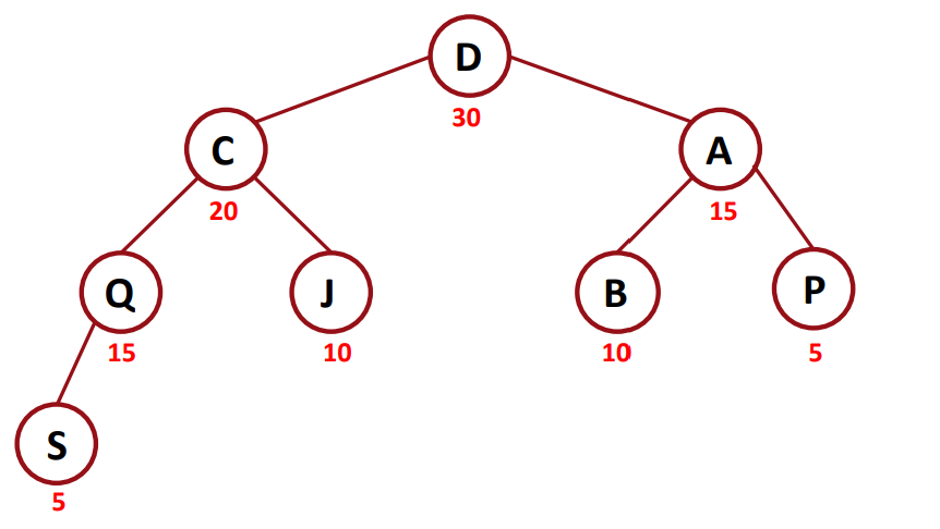
▶ Priority Queue using a Heap
- time complexity to find a task with the highest priority: O(1)
Get (remove) a Largest Value
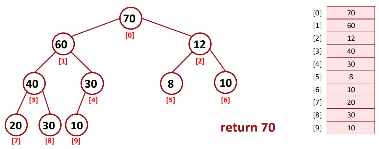

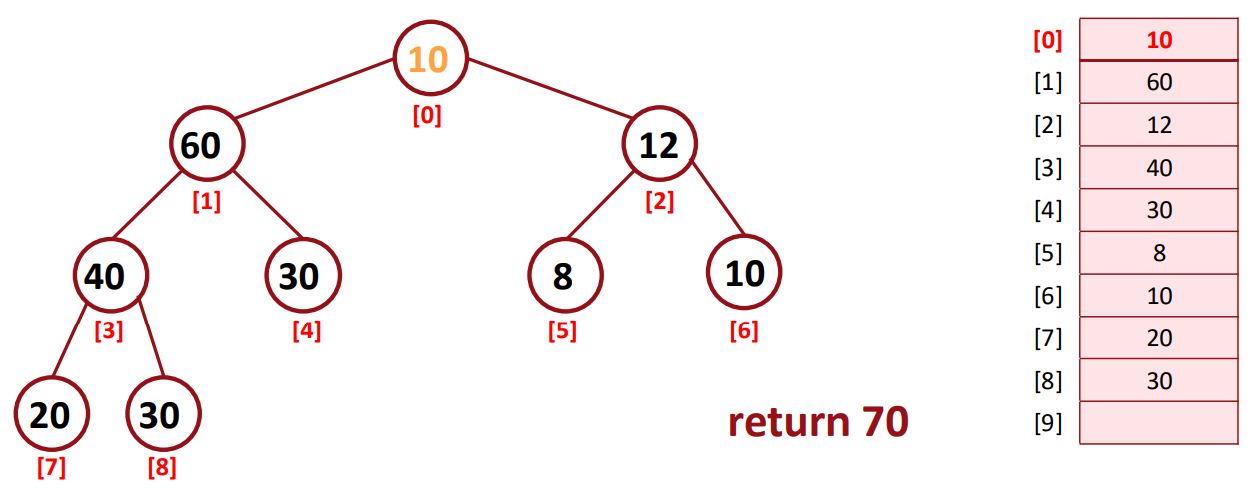
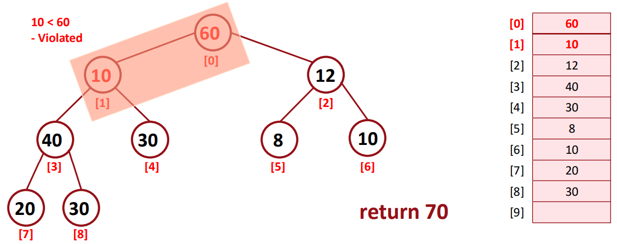
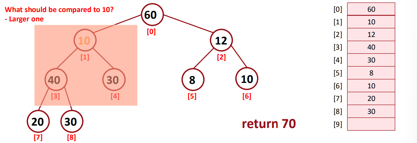
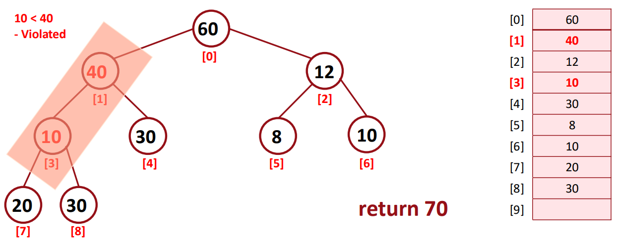

▶ Logical Level
- 1. Copy the bottom rightmost item to the root
- 2. Delete the bottom rightmost node
- 3. Fix the heap property by calling ReheapDown
- Swap nodes if child > parent
- Compare with the lager child node (MAX heap)

▶ reheapDown() - Implementation Level

▶ PQType Definition
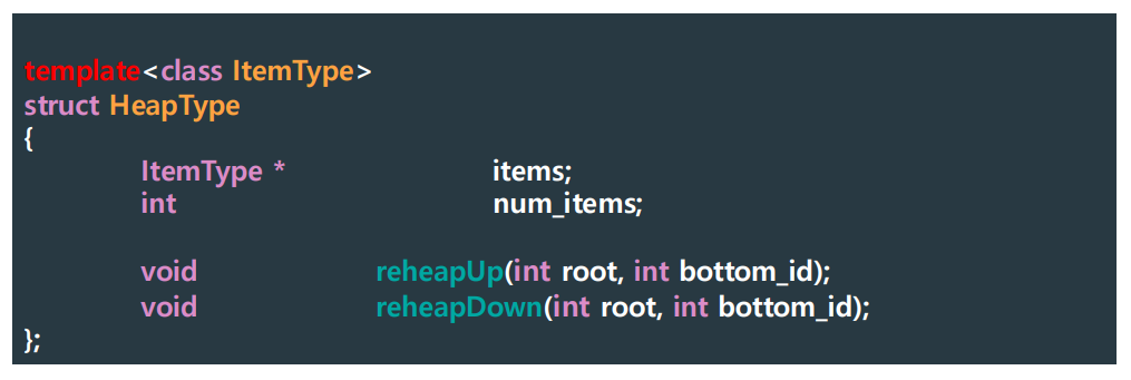
▶ HeapType Definition
- items: 힙이 아이템을 보관하는 array
- num_items: 아이템의 개수
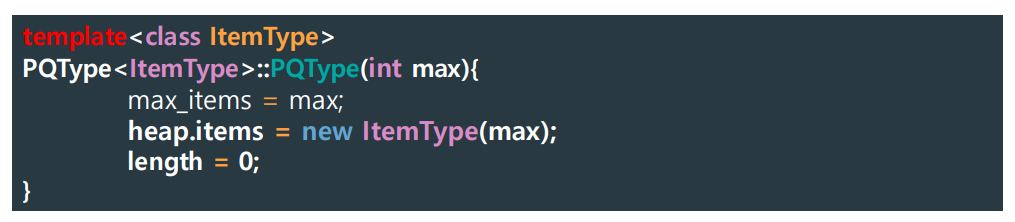
▶ Constructor

▶ destructor & clear()
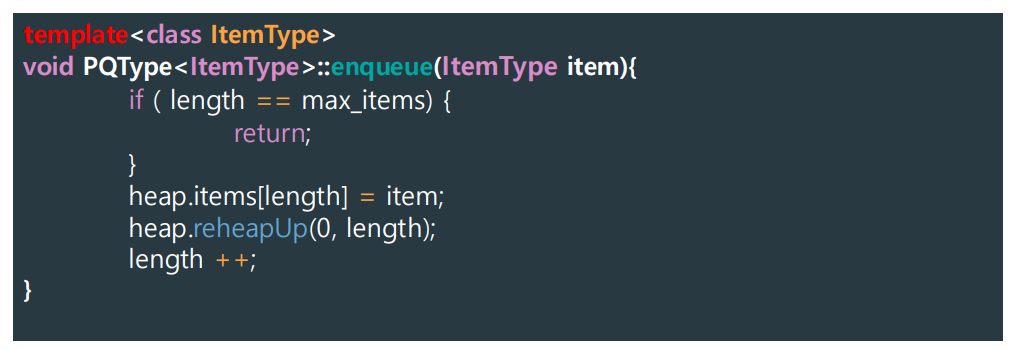
▶ enqueue()
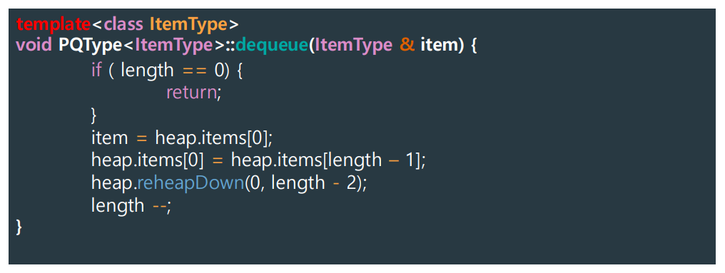
▶ dequeue()
Big-O comparison
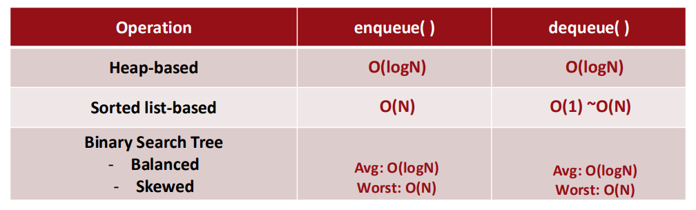
BST는 높이가 랜덤하지만, heap은 완전 이진 트리로 높이가 log N 으로 고정이기에 위와 같은 결과가 나오는 것이다.
- heap의 enqueue는 reheapUp, dequeue는 reheapDown임
그리고 Sorted list의 경우는 array/linked structure, 오름차순/내림차순, 이렇게 4가지 경우의 수가 나올 수 있다.
- enqueue: 모두 O(N)
- dequeue
- array: 오름차순의 경우 O(1), 내림차순의 경우 O(N)
- linked structure: 오름차순의 경우 O(N), 내림차순의 경우 O(1)
이때, enqueue는 특정 item의 위치를 찾아 삽입하는 것이지만, dequeue는 맨 앞(max)의 값을 찾을 필요 없이 제거하니 주의한다.
또한, array의 경우 제거하거나 삽입할 때 한 칸씩 앞으로 당기거나 뒤로 미는 행위를 해야되니 주의해야 한다.
linked structure로 heap 구현 -> 시간복잡도 및 코드 알아야 함!!
Graph
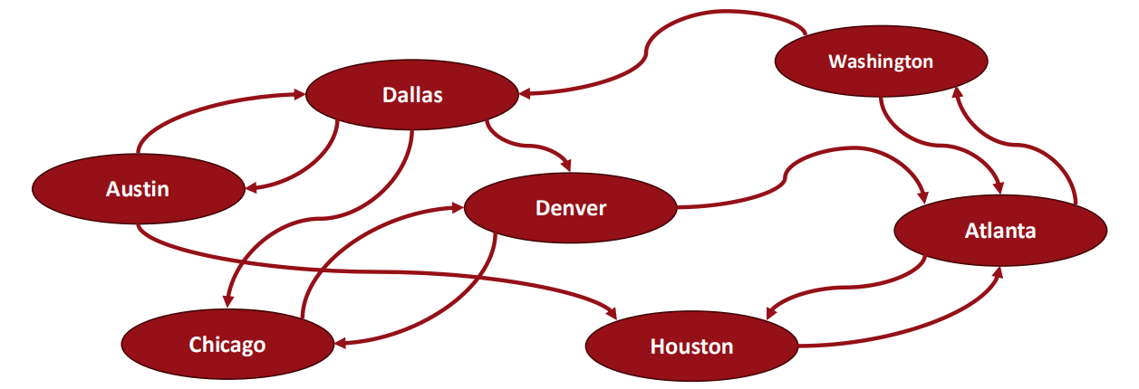
▶ Graph
A data structure that consists of a set of nodes (vertices) and a set of edges that relate the nodes to each other.
THe set of edges describes relationships among the vertices.
Formal Definition
A graph G is defined as floolows:
- G = (V, E)
- V(G): 한 개 이상의 유한한 개수의 노드 집합
- E(G): a sef of edges (pairs of veritces)

▶ Undirected Graph
- the edges in a graph have no direction
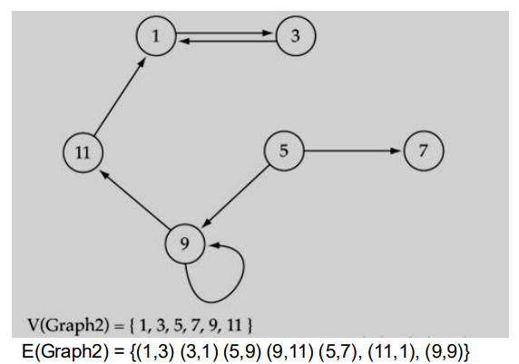
▶ Directed Graph
- the edges in a graph have direction
Directed Graph에서 E(G)를 정의할 때는 vertices의 순서가 중요하니 주의하여야 한다.
- 출발 -> 도착

▶ Tree
Trees are special cases of graphs.
- Acyclic structure: 자기로부터 시작해서 다른 점을 돌아 자기 자신에게 돌아오는 것이 불가능
Terms
- Adjacent nodes: 인접한 노드 (edge로 연결된 노드)
- Path: 특정 노드로부터 다른 특정한 노드까지 이동할 때 지나가는 노드들의 순서
- Complete graph: a graph in which every vertex is directly connected to every other vertex

▶ Complete Directed Graph
- 모든 노드들끼리 직접적으로 연결되어 있어야 함
What is the number of edges in a complete directed graph with N vertices?
- N * (N-1)
- nP2: 시작 정점 N가지 * 도착 정점은 자기 자신을 뺀 N-1가지
-> 공간 복잡도: O(N^2)
※ Big-O는 Upper Bound의 개념으로, 가장 최악의 상황을 감안했을 때의 estimate를 표현해준다. 그리고 이를 시간에 적용하면 시간 복잡도 혹은 메모리를 얼마나 사용하는지를 나타내기 위해 메모리에 적용하면 공간(space) 복잡도가 되는 것이다. 즉, "Big-O = 시간 복잡도"는 아니니 주의하여야 한다.
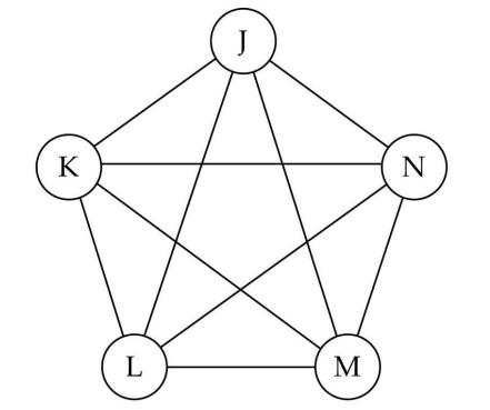
▶ Complete Undirected Graph
- 모든 노드들끼리 직접적으로 연결되어 있어야 함
What is the number of edges in a complete undirected graph with N vertices?
- N * (N-1) / 2
- nC2
-> 공간 복잡도: O(N^2)
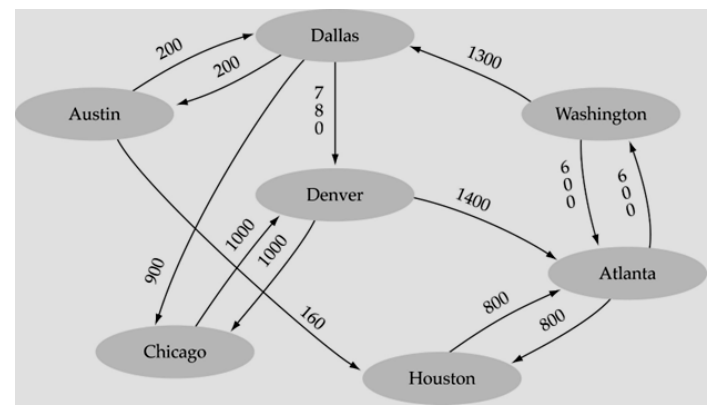
▶ Weighted Graph
- each edge carries a value
graph는 네트워크나 인공지능을 나타내어 분석하는 데에 효과적인 자료구조이다.
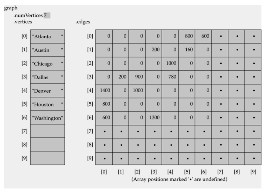
▶ Adjacency Matrix
- 0: edge 존재 X
We can use two matrices to represent a graph (컴퓨터가 이해하기 쉽게 나타냄)
- A 1D array: to represent vertices
- A 2D array (adjacency matrix): to represent the edges

▶ Adjacency List
We can also use a linked list (and on array) to represent a graph
- A 1D array: to represent vertices
- A linked list (adjacency list): to represent the edges

▶ Adjacency Matrix vs. List
- E: edge
- V: vertex
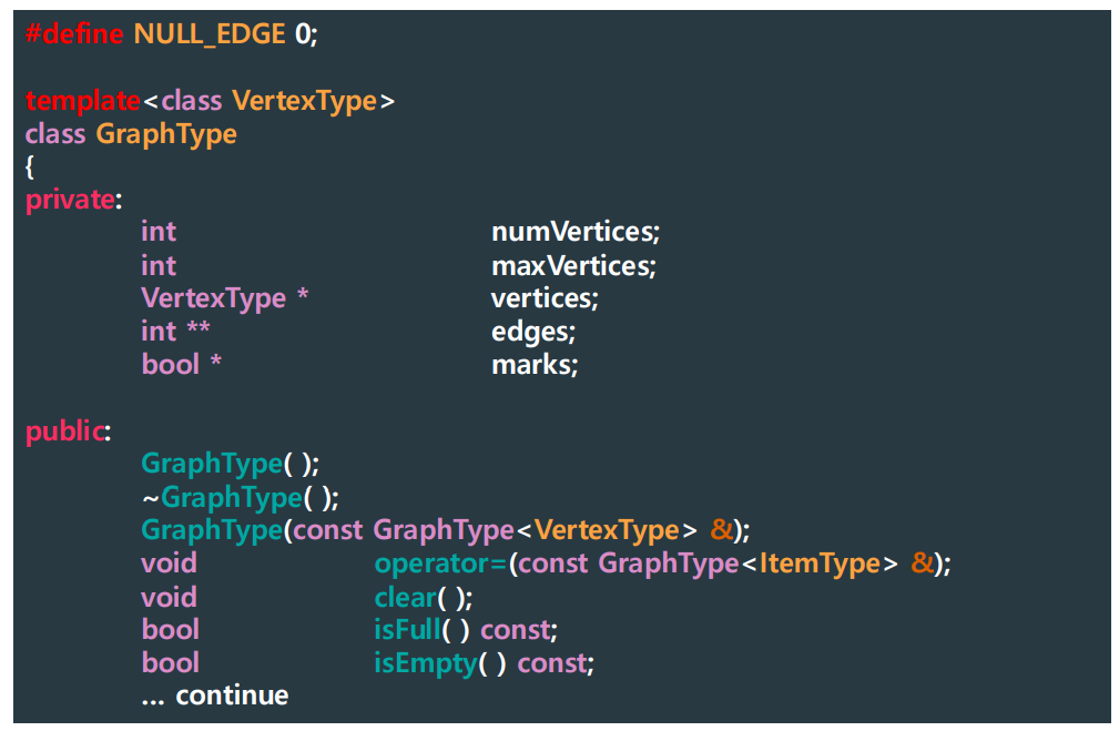
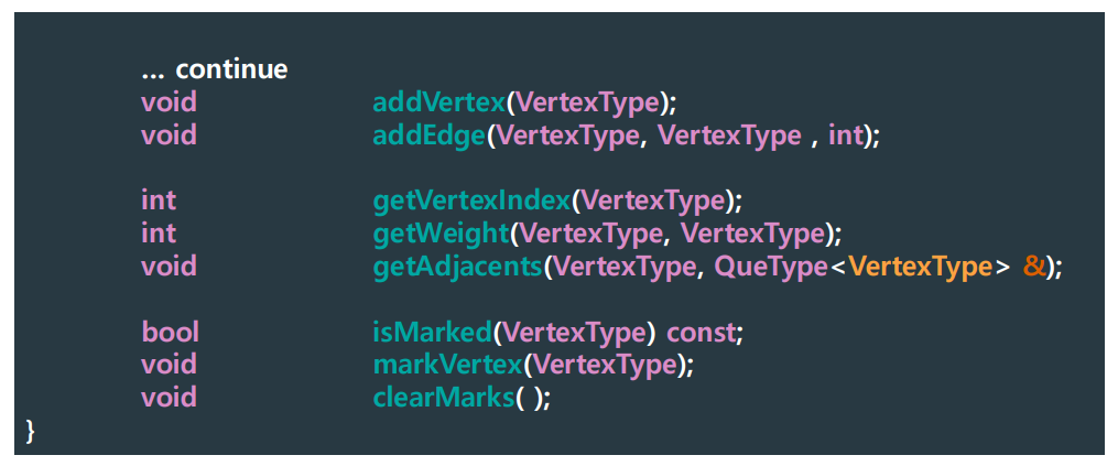
▶ GraphType Definition
- mark: DFS, BFS 할 때 방문 여부를 담는 배열 -> 방문하면 true, 아직 방문 안 했으면 false
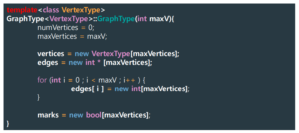
▶ Constructor
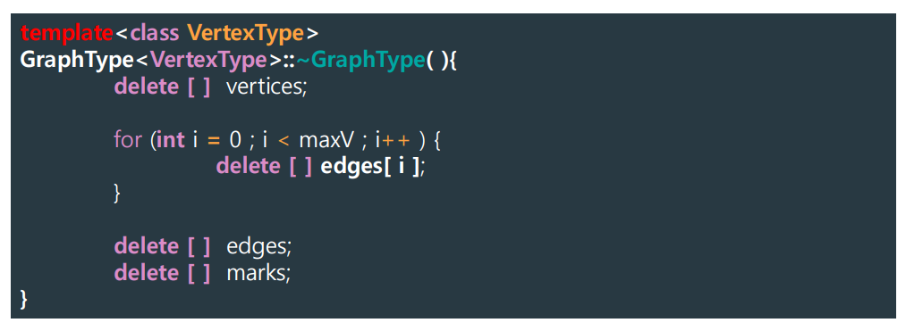
- edge: 더블 포인터 (int 포인터를 가리키는 포인터) -> 2차원 배열
- edges는 int가 아닌 int*들의 배열 -> edges[i]가 i번째 행을 가리키는 포인터 (adjacency matrix)
- 행 할당: edges = new int* [maxVertices];
- 열 할당: for문 -> edges[i] = new int[maxVertices];
▶ Destructor
▶ addVertex()
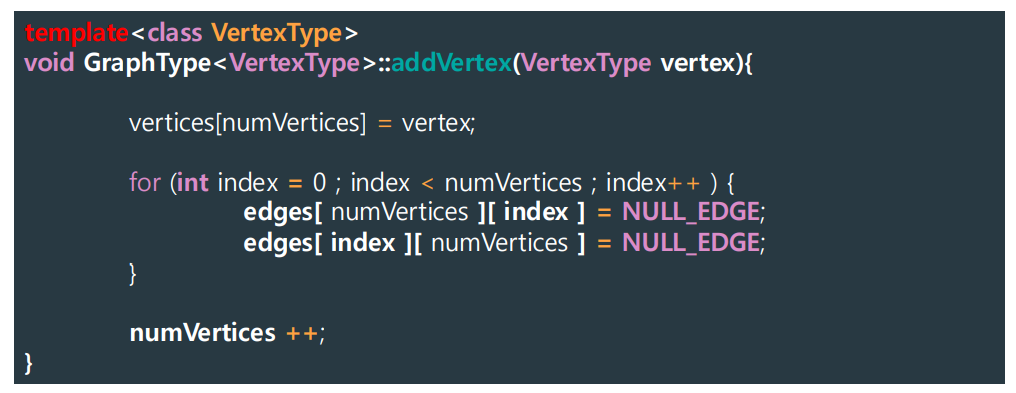
- 새 정점을 vertices의 맨 끝에 넣음
- 새 정점과 "기존 정점들" 사이 간선 초기화
▶ addEdge()
▶ getVertexIndex()

▶ getWeight()
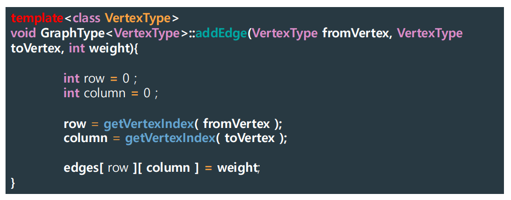
- edges 이차원 배열이 adjacency matrix임
Graph Searching
- 두 노드를 연결하는 path를 찾는 것을 의미
- Methods: Depth-First-Search (DFS) or Breadth-First-Search (BFS)
Depth-First Searching (DFS)
What is the idae behind DFS?
- Visit all in a branch to its deepest point before moving up
- Travel as far as you can down a path
DFS can be implemented efficiently using a stack.


Depth-first Searching (DFS)


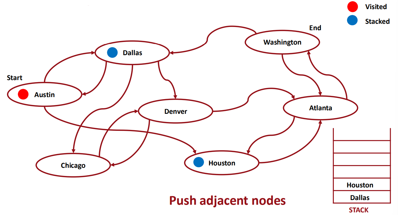

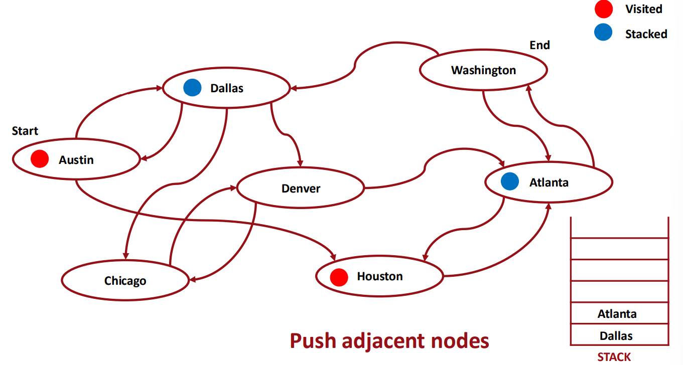

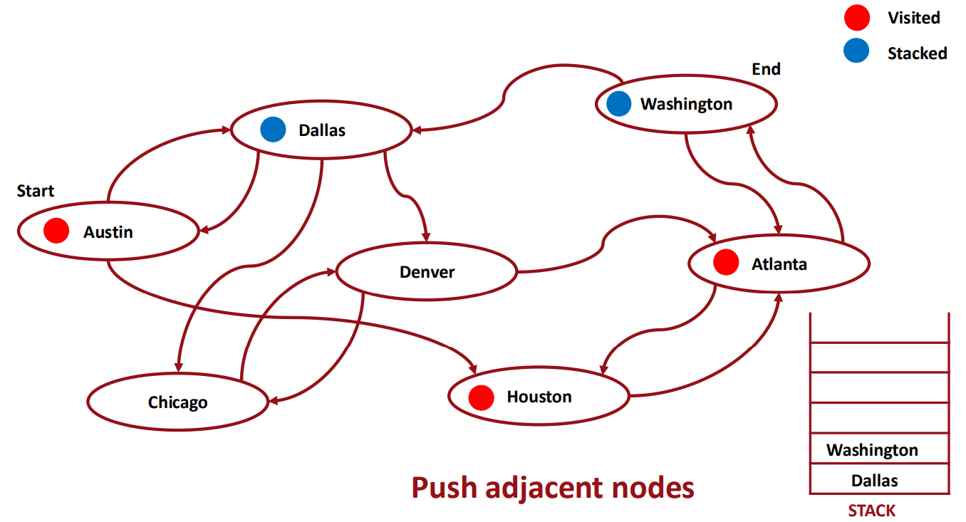
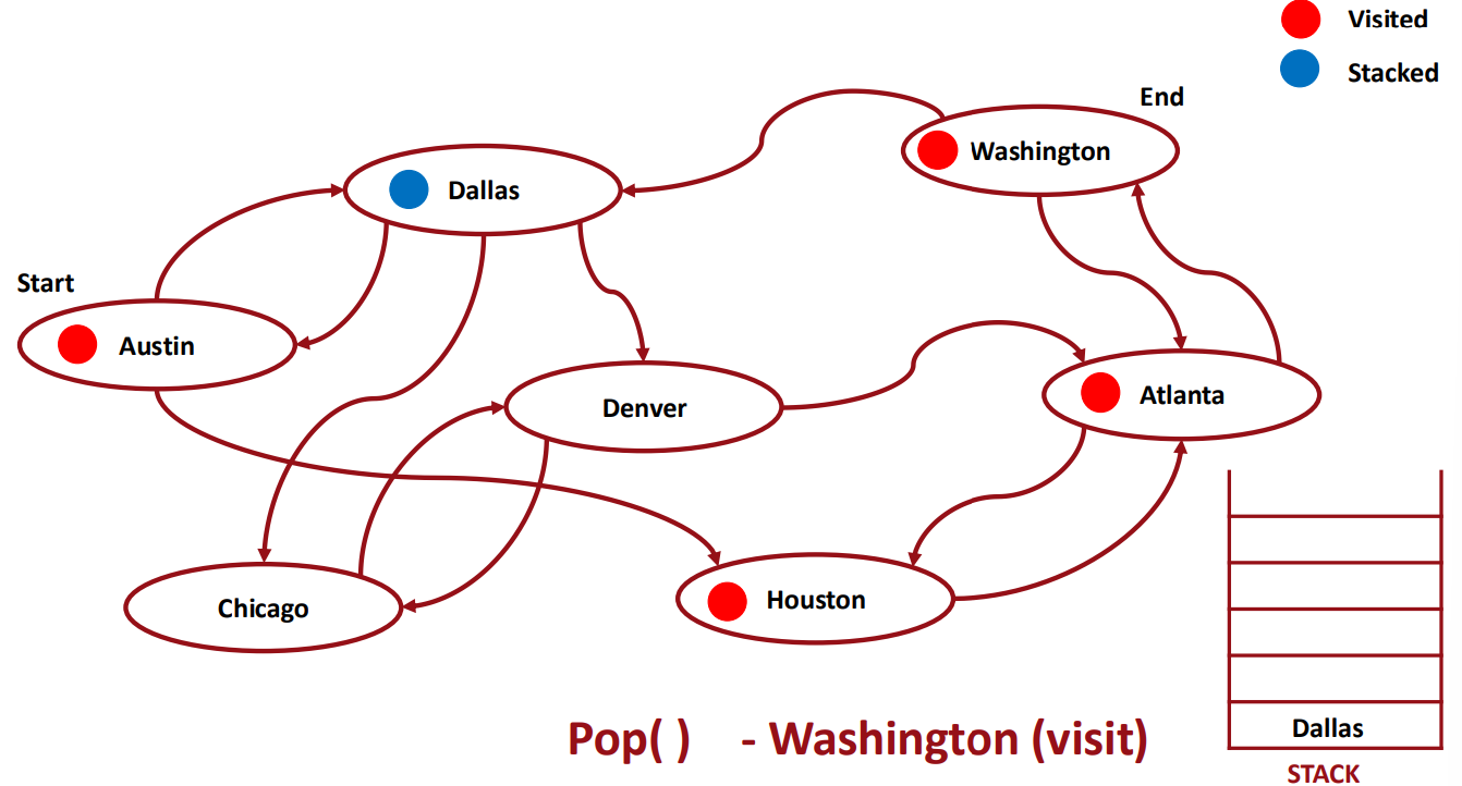
▶ DFS uses STACK
- 1. Pop from Stack
- 2. Visit the popped coordinate (node)
- 3. Push the adjacent coordinates (nodes)
- 4. Repeat 1-3
-> 경로가 있구나! 판단
만약 경로가 없을 경우엔, end를 pop 하지 못했는데 어느 순간 스택이 비어버리게 된다.
-> 경로가 없구나! 판단
Why STACK?
⭐ 스택의 원리가 직전의 상태를 기억해 주는 역할을 하기 때문이다.

▶ DepthFirstSearch()
- 초기화
- DFS
- pop the node
- endVertex에 도달하면 return true
- eddVertex에 도달하지 못했으면 push adjacents
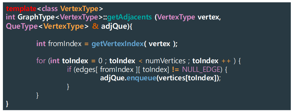
▶ getAdjacents()
⭐ 경로의 합을 구하는 것과, 최단 경로 (weight) 구하는 것과, 경로 출력하는 함수도 만들어 볼 것!
Breadth-First Searching (BFS)
What is the idae behind BFS?
- Visit all nodes on one level before going to the next level
- Look at all possible paths at the same depth before you go at a deeper level
BFS can be implemented efficiently using a queue.
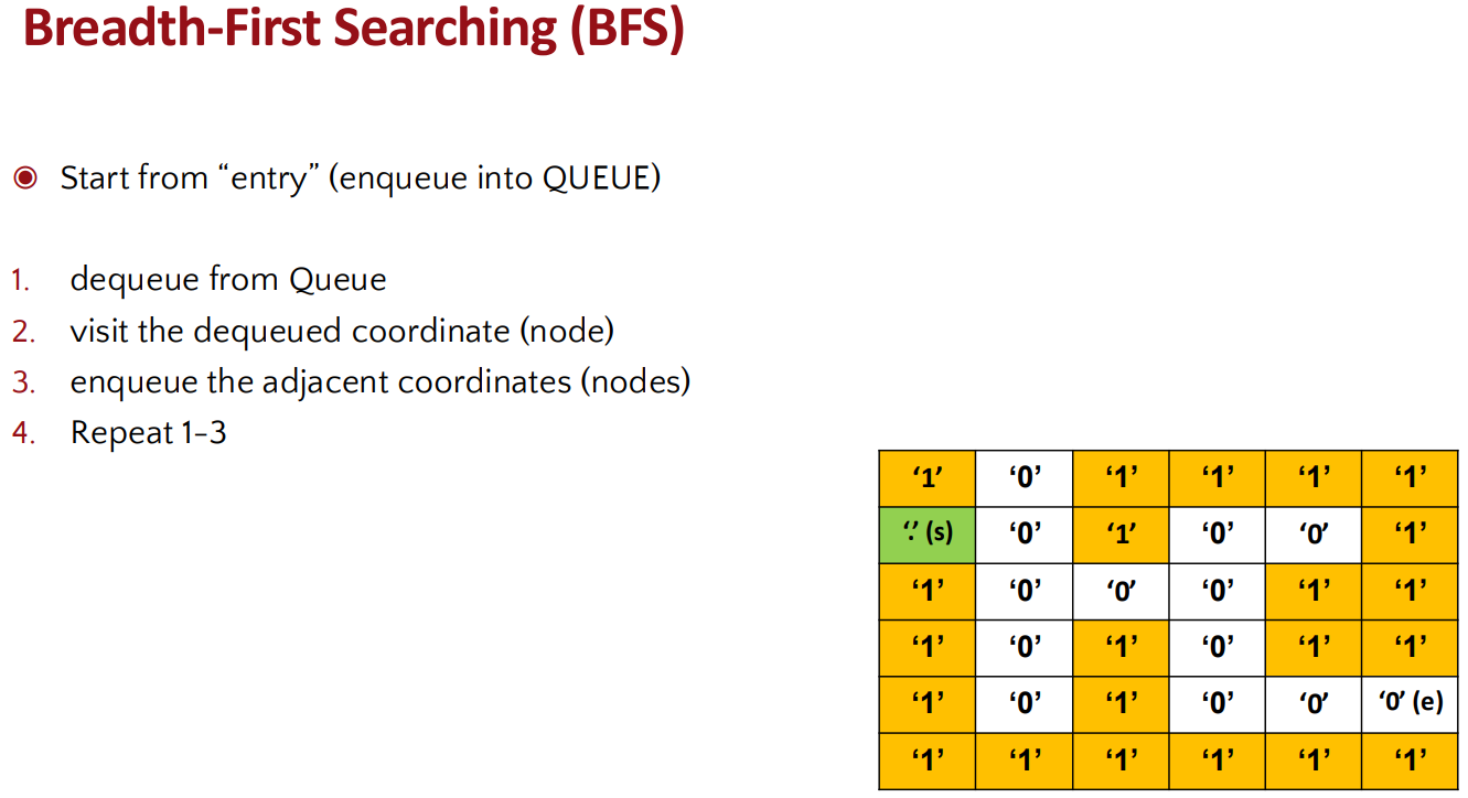
Breadth-First Searching (BFS)
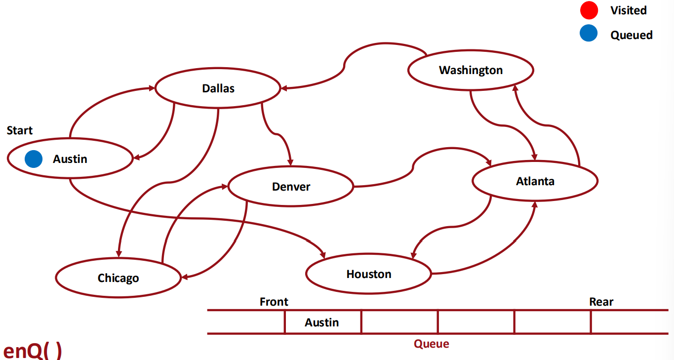

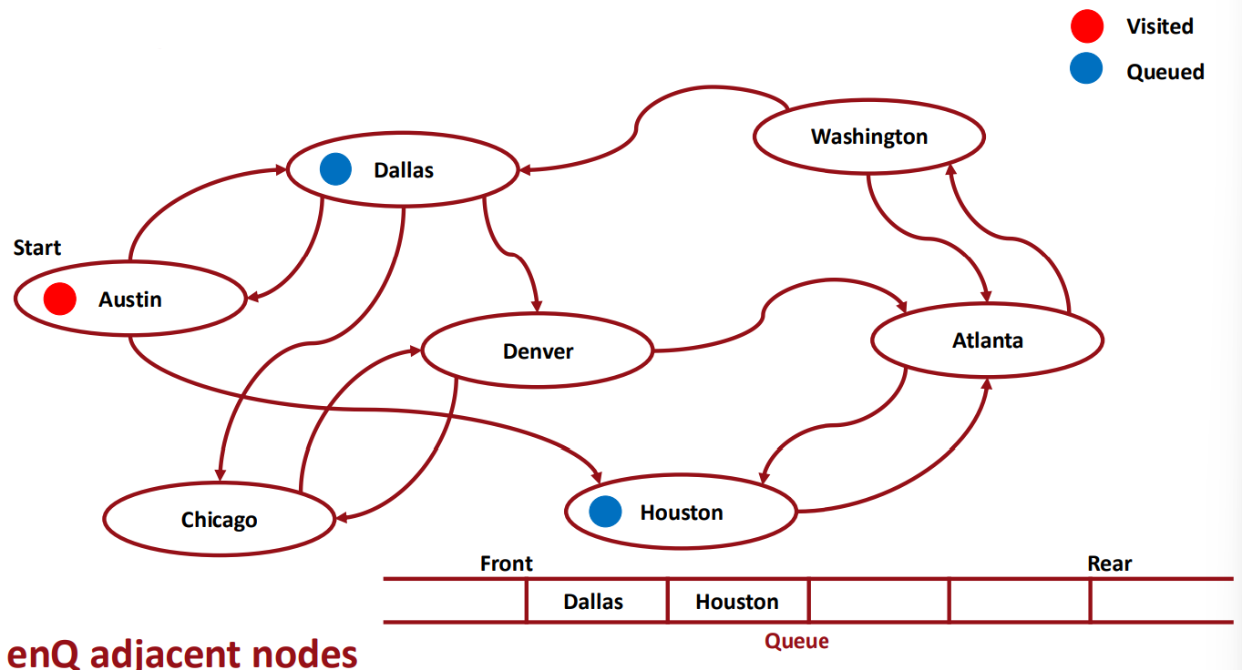
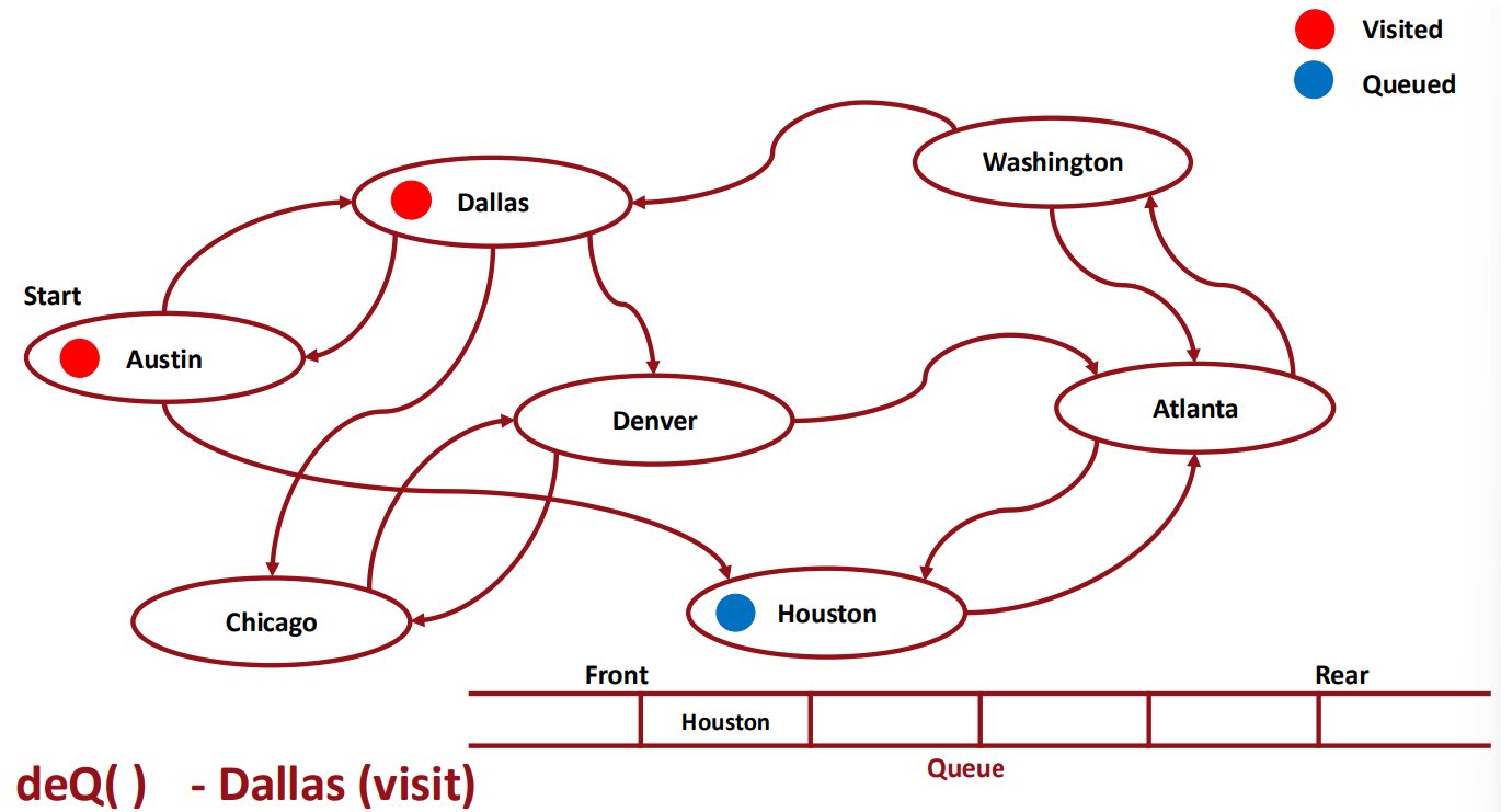
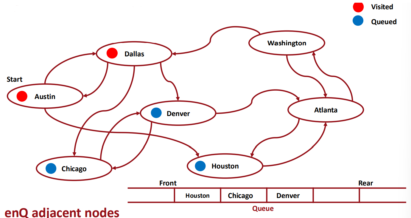
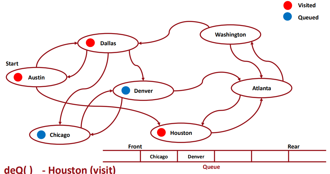

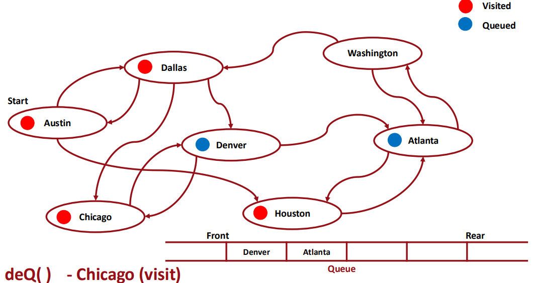
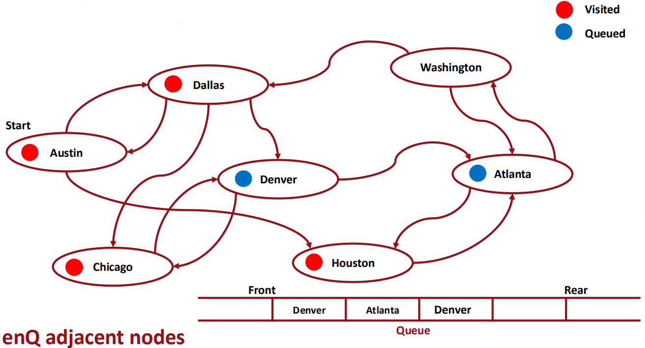
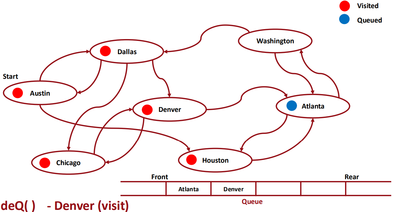
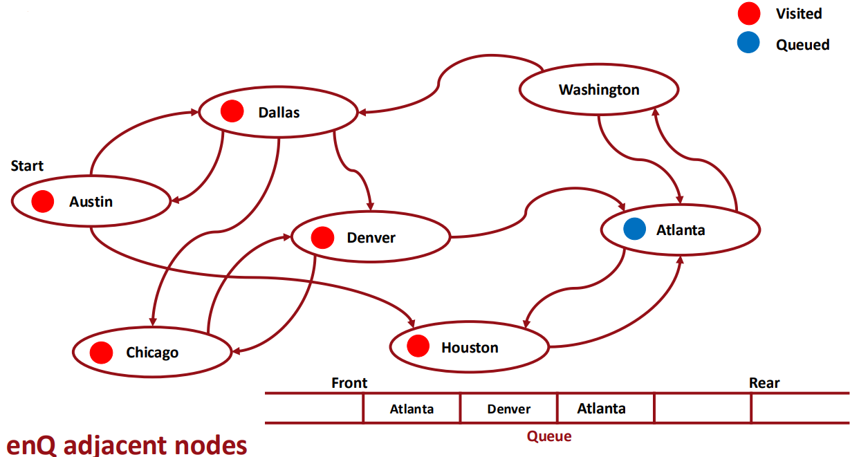
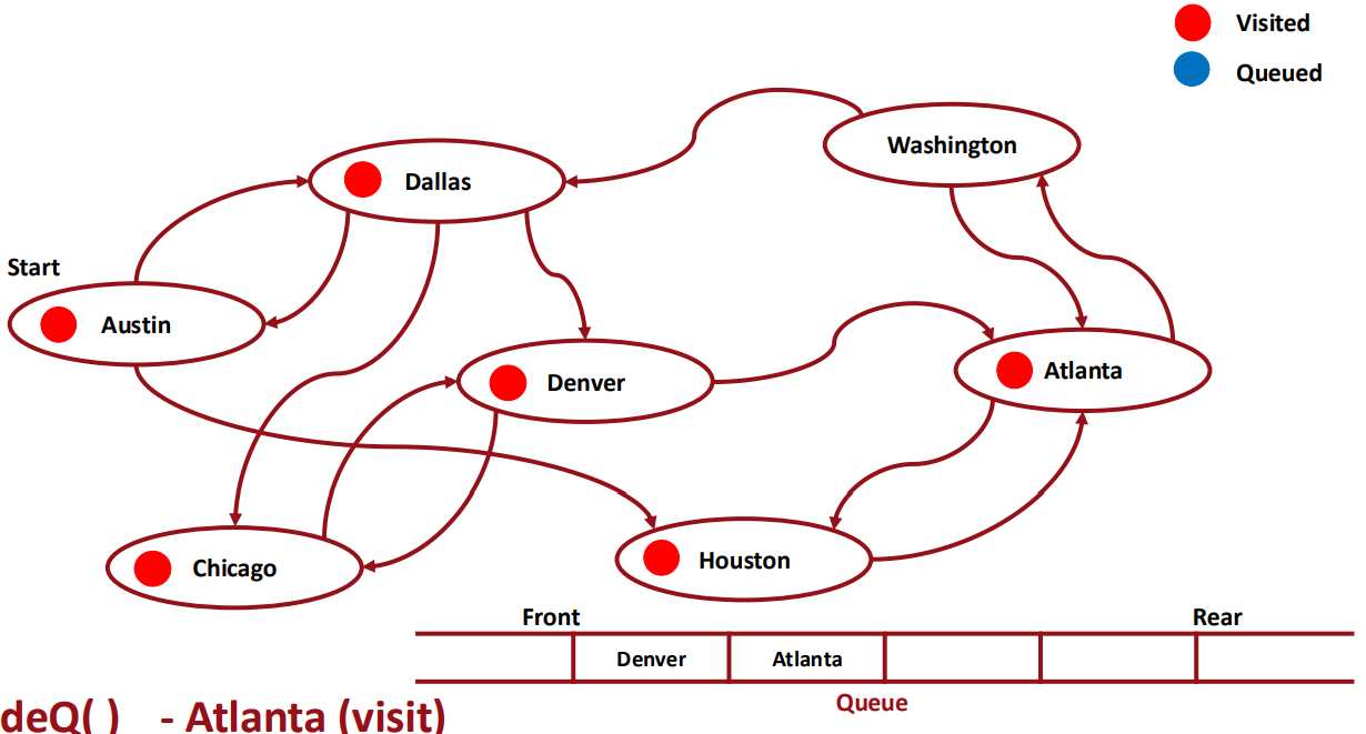


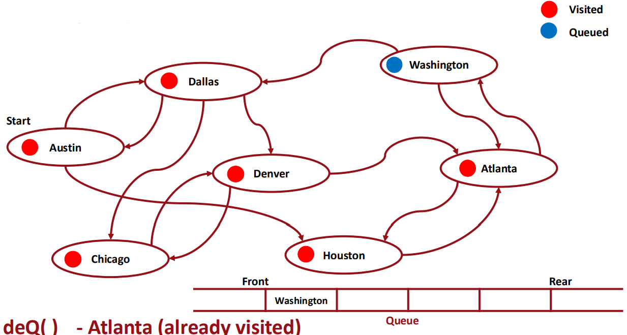

▶ BFS uses QUEUE
- 1. Dequeue from Queue
- 2. Visit the dequeued coordinate (node)
- 3. Enqueue the adjacent coordinates (nodes)
- 4. Repeat 1-3
-> 경로가 있구나! 판단
만약 경로가 없을 경우엔, end를 dequeue 하지 못했는데 어느 순간 큐가 비어버리게 된다.
-> 경로가 없구나! 판단
Why QUEUE?
⭐ 찾아낸 경로가 효율적일 가능성이 BFS보다 높지만, 경로를 찾아내는 과정 자체는 비효율적이다. (DFS와 반대!)
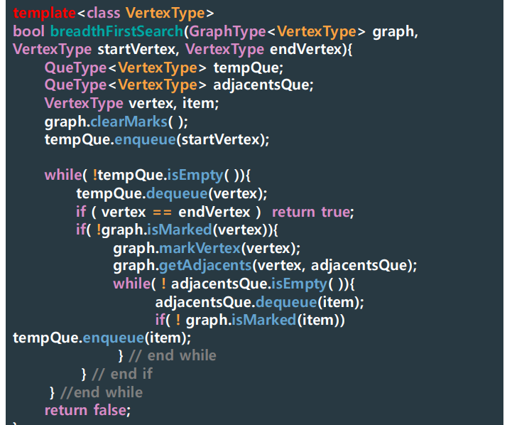
▶ breadthFirstSearch()
⭐ 경로의 합을 구하는 것 해보기!!! (int 반환)
⭐ DFS, BFS 장단점 고민해볼 것!!
Shortest Path Problem
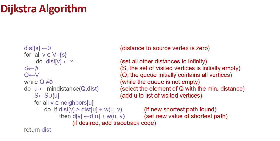

특정한 정점을 출발해서 다른 정점들로 갈 수 있는 최단 경로들의 값을 구해주는 방식
참고자료
https://arsenic-dev.tistory.com/68
Programming Exercise: Lab #3
경희대학교 박제만 교수님의 자료구조 수업을 기반으로 정리한 글입니다.Exercise #1ProblemsImplement rotateFirstItem() in Circular Queue with Reserved space.This function "ROTATES" the first item of the queue.▶ Both are OKAY (in
arsenic-dev.tistory.com
'CS > 자료구조' 카테고리의 다른 글
| Programming Exercise: Lab #7 (1) | 2025.06.08 |
|---|---|
| Chapter 8: Tree (2) | 2025.06.08 |
| Programming Exercise: Lab #6 (3) | 2025.06.02 |
| Chapter 7: Recursion (0) | 2025.06.02 |
| Programming Exercise: Lab #5 (0) | 2025.05.20 |